Parametric
Estimation

MLE and hypothesis testing

Yu Cheng Hsu

Intended learning outcomes

• Define and formulate the likelihood function (\(\mathcal{L}_n(\theta)\)) as the joint density of IID observations
• Differentiate between MLE and Maximum A Posteriori (MAP) estimates, specifically how MAP incorporates a Bayesian prior
• Understand different hypothesis testing approach

Estimating distribution parameter from data

• In this session we focus on how to estimate the distribution parameters from the IID observed data \(X=x_1,\dots,x_n\)
• We assume \(X\) follows a specific distribution how can we know the paparemeter?
  • If it follows a normal distribution, then what is the procedure

Intuitive guess

Using the sample mean, variance as the best guess

Likelihood

The likelihood function (\(\mathcal{L}_n(\theta)\)) is the joint density of IID observations \(X=x_1,\dots,x_n\) with PDF \(f(x;\theta)\), treated as a function of the parameter \(\theta\) given the fixed data.

\(\mathcal{L}_n(\theta)=\prod_{i=1}^nf(x_i|\theta)\)

• Likelihood is the product of the probabilities of observing \(X\) as a function of different \(\theta\).
• This is the observed data we see in calculating Bayesian posterior

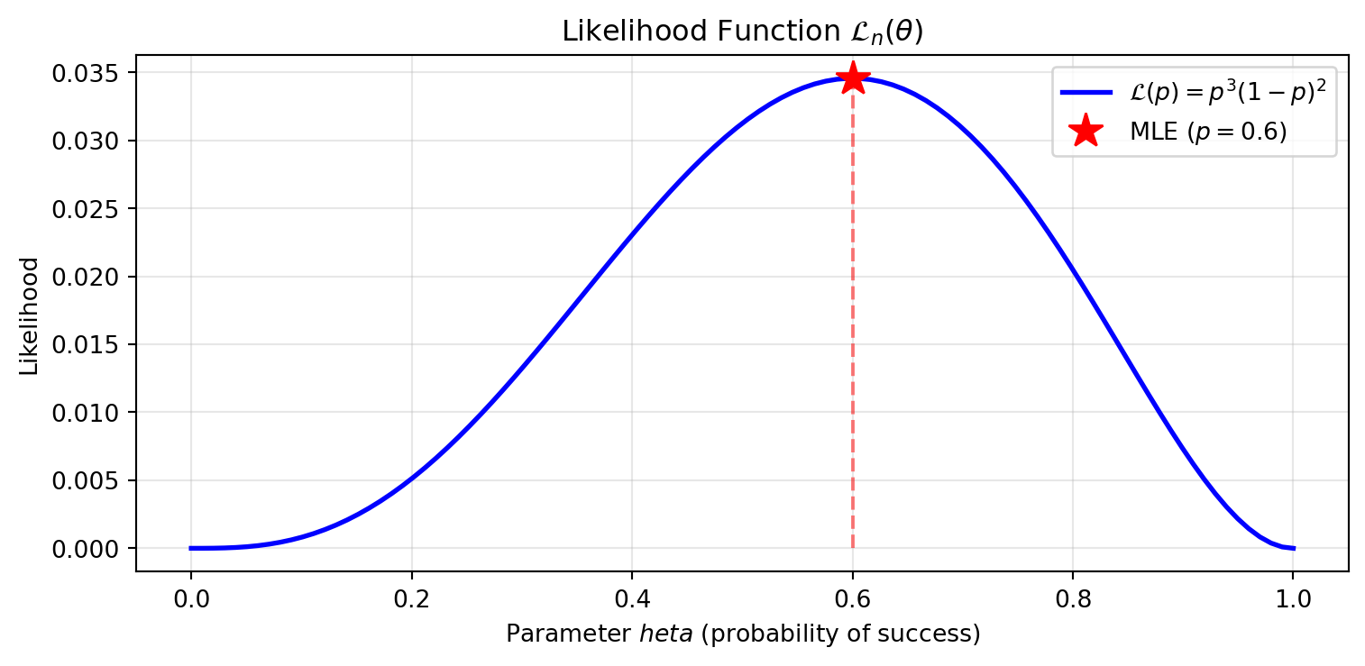
Example if \(X \sim \text{Bern}(p)\), and we observed \([1,0,0,1,1]\)

then the likelihood is

\[ \mathcal{L}_n(\theta) = p^3(1-p)^2 \]

Maximum likelihood

• The ideal \(\theta\) is the one (\(\hat{\theta}\)) that maximizes the likelihood (i.e., makes the observed data most probable). We call this the Maximum Likelihood Estimate (MLE).
• Calculus tells us the maximum of a function occurs where:

\(\small\frac{d\mathcal{L}_n(\theta)}{d\theta}=0 \quad \text{and} \quad \frac{d^2\mathcal{L}_n(\theta)}{d\theta^2}<0\)

Calculation notes

1. Any positive constant multiplier \(c\) won’t affect the location of the maximum, so constants can be ignored.
2. Taking the logarithm of the likelihood is often easier for calculation. We define the log-likelihood function as \(\ell_n(\theta)=\ln(\mathcal{L}_n(\theta))\). Reasons:
   1. Numerical stability
   2. Logarithms transform products into sums.

Example: Bernoulli MLE

if \(X \sim \text{Bern}(p)\), and we observed \([1,0,0,1,1]\)

we would like to maximize the likelihood

\[ \begin{aligned} \max_\theta\mathcal{L}_n(\theta) =& \max_\theta p^3(1-p)^2\\ \frac{d\mathcal{L}_n(p)}{dp} =& p^2(5p^2-8p+3) =0 \\ p = & 0,0.6, \text{or } 1 \\ \frac{d^2\mathcal{L}_n(p)}{dp^2} =& 20p^3-24p^2+6p \\ \mathcal{L}^{''}_n(0) = 0 , & \mathcal{L}^{''}_n(0.6) = -0.72, \\ \mathcal{L}^{''}_n(1) =& 2 \end{aligned} \]

import numpy as np
import matplotlib.pyplot as plt

def likelihood(p):
    """
    Likelihood function for Bernoulli(p) with data [1, 0, 0, 1, 1].
    L(p) = p^3 * (1-p)^2
    """
    return (p**3) * ((1 - p)**2)

# 1. Setup the grid
p_values = np.linspace(0, 1, 100)
L_vals = likelihood(p_values)

# 2. Find MLE for visualization
mle_p = 0.6
mle_val = likelihood(mle_p)

# 3. Create the Plot
plt.figure(figsize=(8, 4))

# Plot the curve
plt.plot(p_values, L_vals, 'b-', lw=2, label=r'$\mathcal{L}(p) = p^3(1-p)^2$')

# Mark the MLE
plt.plot(mle_p, mle_val, 'r*', markersize=15, label=f'MLE ($p={mle_p}$)')
plt.vlines(mle_p, 0, mle_val, colors='r', linestyles='dashed', alpha=0.5)

# Formatting
plt.title(r'Likelihood Function $\mathcal{L}_n(\theta)$')
plt.xlabel('Parameter $\theta$ (probability of success)')
plt.ylabel('Likelihood')
plt.legend()
plt.grid(True, alpha=0.3)
plt.tight_layout()

plt.show()

The MLE estimation is 0.6, which is exactly the sample mean

Maximum A Posteriori (MAP) Estimate

• The idea of maximizing \(p(\theta|x)\) is called maximum a posteriori (MAP) estimate, the problem has the following format

\[ \begin{aligned} \hat{\theta}_{MAP}= &\arg\max_\theta p(\theta|x) = \arg\max_\theta \frac{p(x|\theta)p(\theta)}{\int_\Theta p(x|\theta)p(\theta)d\theta} \\ = & \arg\max_\theta p(x|\theta)p(\theta) \end{aligned} \]

Implication

• MAP is the mode of the posterior distribution.
• It acts as a bridge between Frequentist MLE and full Bayesian inference.

Example: Bernoulli MAP

if \(X \sim \text{Bern}(p)\), and we observed \([1,0,0,1,1]\), We have a prior on \(p\sim \text{Beta}(2,2)\)

What is the MAP estimate of \(p\)

Hardcore calculus

\[ \begin{aligned} \arg\max_p p(p|x) & = \arg\max_p p^3(1-p)^2 \cdot p^{2-1}(1-p)^{2-1} \\ \frac{d}{dp} [p^4(1-p)^3] &= 4p^3(1-p)^3 - 3p^4(1-p)^2 \\ & = p^3(1-p)(p-1)(7p-4) =0 \\ p & = 0, 1, 4/7 \\ \text{Second derivative test confirms} & \text{ maximum at } p = 4/7 \end{aligned} \]

Example: Bernoulli MAP

Using Conjugate Priors

\[ \begin{aligned} p(p|x) & \sim \text{Beta}(\alpha', \beta') \\ \alpha' &= \alpha + \sum x_i = 2 + 3 = 5 \\ \beta' &= \beta + (n - \sum x_i) = 2 + 2 = 4 \end{aligned} \]

The MAP (mode) for \(\text{Beta}(\alpha, \beta)\) is \(\frac{\alpha-1}{\alpha+\beta-2} = \frac{5-1}{5+4-2} = \frac{4}{7} \approx 0.57\).

Takeawys

MLE

• Maximizes the probability of the data given parameters: \(p(x|\theta)\).
• For common distributions, MLE often corresponds to:
  • Sample mean (\(\bar{x}\))
  • Sample variance (\(s^2\))
• Guaranteed to have asymptotic properties (consistency and efficiency) as \(n \to \infty\).

MAP

Maximizing the posterior (observed data+ prior)

\[ p(\theta|x)\propto p(x|\theta)p(\theta) \]

• MLE only maximize the \(p(x|\theta)\) without considering \(p(\theta)\)
• Intuitively, the \(p(\theta|x)\) has the maximum at the posterior mean
• Not the optimal estimation but incorporate with prior

Statistical inference

Preface

• This topic is highly correlated with BIOF2013, but we will focus more on the underlying mechanics of why these tests work.
• In BIOF2013, we have introduced several hypothesis test methods

Hypothesis test image link

The Wald Test

Considering a two-tailed test

\[ H_0=\theta=\theta_0 \text{ v.s. } H_1=\theta\neq\theta_0 \]

Assumes \(\hat{\theta}\) is asymptotically Normal

\[ W=\frac{\hat{\theta}-\theta_0}{\hat{se}}\leadsto N(0,1) \]

Important thing

• Requires sufficient sample size for the CLT to ensure \(\hat{\theta}\) is asymptotically Normal.
• The p-value is \(P(|W| \geq |W_{obs}| \mid H_0)\), not the probability that the null hypothesis is true.

Likelihood ratio test (LRT)

A more general way incorporating for a multivariate parameters (i.e. a vector-based parameter \(\theta=(\theta_1,\dots,\theta_n)\)) is likelihood ratio test. The general form is

\[ H_0=\theta\in\Theta_0 \text{ v.s. } H_1=\theta\notin \Theta_0 \]

The test statistics

\[ \Lambda = -2\ln\left(\frac{\mathcal{L}(\hat{\theta}_0)}{\mathcal{L}(\hat{\theta})}\right) \leadsto \chi^2_{df} \]

Implication

• Likelihood ratios provide a powerful framework for comparing nested models.
• This method can be used in test regression
• Asymptotic assumption

Application of LRT

• Chi-square test on 2x2 contingency table
  • We can treat each cell as multinomial distribution outcome
  • We are simultaneously estimating 2 probability on two variables
• Multinomial distribution parameter hypothesis testing
• Regression: goodness-of-fit test

Discussion question

Why do we use Fisher’s exact test instead of the \(\chi^2\) test for small sample sizes?

Comparison of LRT and Wald Test

• In a single parameter setting, both Wald test and LRT have similar power and results.

Comparison of LRT and wald test image Link

Discussion question

What are the difference of Wald test with multiple comparison correction and LRT?

Permutation test

The permutation test is a non-parametric method with minimal assumptions about the underlying distribution.

• Suppose that \(X \sim F_X\) and \(Y \sim F_Y\)
• The hypothesis is \(H_0: F_X = F_Y, H_1 \neq F_Y,\)
• Observed samples \(x_1,\dots, x_m\) and \(y_1,\dots, y_n\).
• Test statistic \(T_{obs} = |\bar{x}_m - \bar{y}_n|\).

Procedure

1. Compute the observed test statistic \(T_{obs}\).
2. Randomly shuffle (permute) the group labels many times (\(B\)).
3. Calculate the statistic \(T_j\) for each permutation.
4. The approximate p-value is \[ \frac{1}{B}\sum_{j=1}^B I(T_j \geq T_{obs}) \]